8 min to read
How I Used a Convolutional Neural Network to Classify Cricket Shots

I’ve recently delved into the world of deep learning; more specifically, image classification.
After completing the first lecture in the fast.ai MOOC, I decided to play around a little with their library. This led me to make a model that could classify different types of cricket shots.
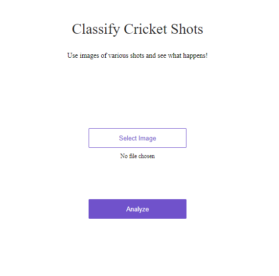
Try it out at Classify Cricket Shots. The model is not perfect, but it does have an accuracy rate of 96%.
 My image classifier web app!
Setting Up Prerequisites
For this model, I used Google Colab to host my notebooks.
The first step in this process is to go to https://colab.research.google.com/ and sign in with your Google account.
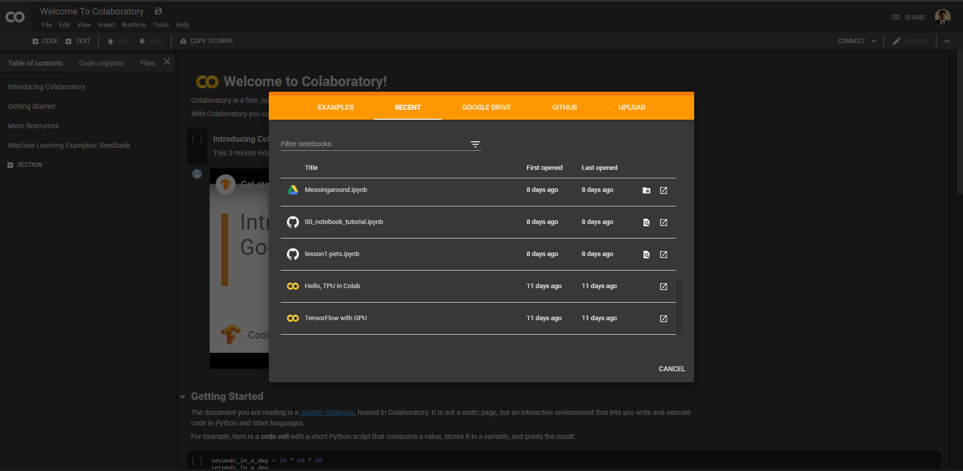
You should be presented with a screen that looks similar to this:
 Google Colab Welcome Screen
If you want to follow along with this tutorial, you should open the notebook in my GitHub repository in Colab, by following the steps below.
To open the notebook from my GitHub repository, click on the GitHub tab, and type in: siddhantdubey.
 This is the screen that pops up
Next, click on the typesofshots.ipynb file. Don’t worry about the error messages that pop up throughout the notebook, we will take care of those.
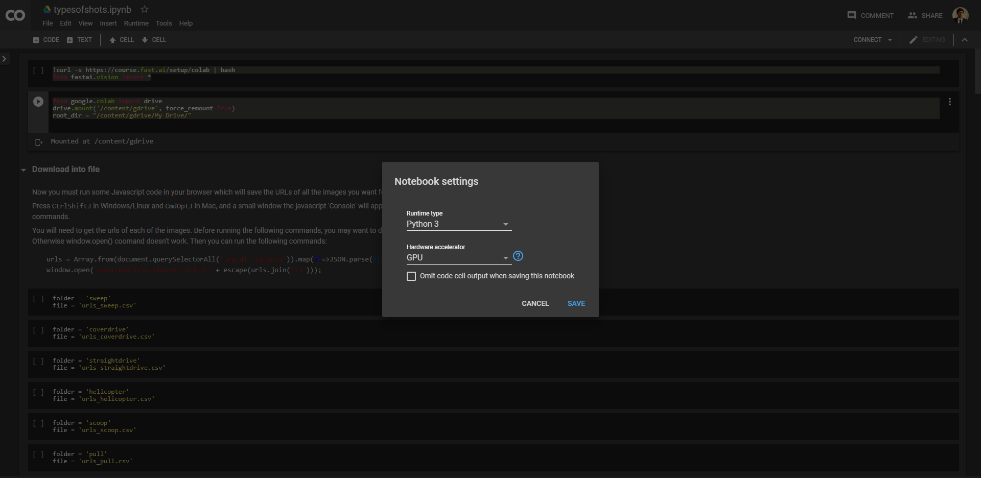
To make sure your notebook will use a GPU accelerator, click runtime on the top tab, and then click change runtime type in the drop-down menu.
You should see this on your screen:
 Notebook settings
Choose GPU as your hardware accelerator and we are good to go.
Writing the Code
Most of the code throughout this tutorial will be getting and cleaning the data. In addition, I will be focusing more on how to make it work, and not on why it works.
The first step is to import the library we need.
!curl -s https://course.fast.ai/setup/colab | bash
from fastai.vision import *
Run that block of code in the notebook to download and import the fast.ai vision library.
The next step is to make sure that the notebook saves the data necessary to your drive, and is able to import data as well.
To do this, run the following block of code:
from google.colab import drive
drive.mount('/content/gdrive', force_remount=True)
root_dir = "/content/gdrive/My Drive/"
This will ensure that your data is nice and usable.
Now comes the time to actually download the data!
We will get images for six types of cricket shots:
-
The sweep.
-
The cover drive.
-
The straight drive.
-
The helicopter shot.
-
The scoop shot.
-
The pull shot.
There are more types, and you can definitely experiment with those as well after this tutorial.
Type in the search query you want, in this case, “cricket sweep shot”), replacing “sweep shot” by each type of cricket shot you want.
Then press Ctrl+Shift+J in Windows/Linux and Cmd+Opt+J in Mac, and a small window (the JavaScript ‘console’) will appear.
That is where you will paste the JavaScript commands:
urls = Array.from(document.querySelectorAll('.rg_di .rg_meta')).map(el=>JSON.parse(el.textContent).ou);
window.open('data:text/csv;charset=utf-8,' + escape(urls.join('\n')));
Copy and paste that into the console, and it should start the downloading the images.
Rename the download file to urls_sweep.csv where “sweep” is the name of any of the shots, without spaces or capitalization.
Next, create a folder in your google drive called data and within that folder create another folder named shots.
Upload all the CSV files you get into the shots folder.
The next steps must be followed in this exact order!
-
Run this code block.
folder = ‘sweep’ file = ‘urls_sweep.csv’
-
Run this code block.
path = Path(root_dir + ‘data/shots’) dest = path/folder dest.mkdir(parents=True, exist_ok=True)
-
Run this code block.
classes = [‘sweep’, ‘coverdrive’, ‘straightdrive’, ‘helicopter’, ‘scoop’, ‘pull’]
-
Run this code block.
download_images(path/file, dest, max_pics=1000)
Repeat these four steps for each of the folders’ file blocks, so six times in total.
Next, run the following block of code:
for c in classes:
    print(c)
    verify_images(path/c, delete=True, max_size=500)
#This deletes all the images that it cannot open
What we have just done, is create folders for each of the different types of shots, and then we download the images from the CSV files into said folders.
Create the Dataset
Now we have to create the dataset itself.
To do so run the following block of code:
np.random.seed(42)
data = ImageDataBunch.from_folder(path, train=".", valid_pct=0.2,
        ds_tfms=get_transforms(), size=224, num_workers=4).normalize(imagenet_stats)
This creates a dataset from our path, which is data/shots, and it transforms all the pictures into an image that is 224x224.
Why 224x224? Well, it makes it easier for the model to read and easier for us to code.
Running the following two code blocks will show us our classes (labels) and some of the images in our dataset.
data.classes

data.show_batch(rows=3, figsize=(7,8))
Next, run this code block for more info on the size of our dataset:
data.classes, data.c, len(data.train_ds), len(data.valid_ds)
Training the Model
We are finally ready to train our model!
This is the shortest step of the process in terms of code, but it has the potential to be the longest in terms of time. Not because it is hard to code, but because of how much processing power it requires.
If you tried to do this on your computer instead of on an external host like Google Colab, it would take much longer.
To begin, run the following block of code:
learn = cnn_learner(data, models.resnet50, metrics=error_rate)
This creates a convolutional neural network using the ResNet-50 model. ResNet-50 is currently one of the, if not the, best image recognition models.
Next, run this block of code to train the network.
learn.fit_one_cycle(5)
This trains the model for five ‘epochs’ and shows you what the error rate is in each cycle.
Run the following blocks of code to save the model, and also learn when it is most efficient.
learn.save('stage-1')
learn.unfreeze()
learn.lr_find()
learn.recorder.plot()
This will save the model, unfreeze it for further training and plot how efficient it is to train.
learn.fit_one_cycle(2, max_lr=slice(3e-5,3e-4))
By running the above code block, we improve the accuracy of the model and could potentially push it past 96% accuracy by training it for more epochs, like five, instead of the current two, epochs. This is up to you.
To save the model once more, run the following block of code:
learn.save('stage-2')
Interpreting the Data
First, we need to load the model to look at how good it is.
learn.load('stage-2');
Train it one more time for one epoch.
learn.fit(1)
To get the interpretation of the model’s effectiveness run the following code block:
interp = ClassificationInterpretation.from_learner(learn)
To show the confusion matrix, which shows you how many times the images in each category were matched with the correct labels, run the following block of code.
interp.plot_confusion_matrix()
The diagonal from the top left corner to the bottom right corner showcases how often each image was identified correctly.
To see which images were most confused with each other (my personal favorite statistic), run the following block of code:
interp.most_confused()
To plot the top losses — the images the model was most confident about, but then got wrong anyway — run this block of code:
interp.plot_top_losses(9, figsize=(15,11))
And we are done! If you wish to export your model for production as a web app and further test it, keep reading.
Exporting Your Model
Run the following lines of code:
learn.export()
defaults.device = torch.device('cpu')
learn = load_learner(path)
This should save an export.pkl file to your Google Drive in the data/shots directory.
After you do this, do not train your model again or it will include shots as one of the classes to train for.
To turn this model into a web app, follow this very short and easy tutorial. This will help you publish your model (hopefully not this exact one) as a web app, like mine. It takes around 10 minutes and is very easy.
Comments